1. Introduction
a) The Scientific Process
Climate scientists, like other scientists, use a cyclical process to advance their understanding. Usually it starts with a question, a lack of understanding. They form hypotheses based on previous knowledge or experience. Formulating a good hypothesis is usually not trivial. A useful hypothesis must be testable. That is, there must be the possibility to obtain evidence that confirms or falsifies the hypothesis. In climate science the evidence is most often quantitative data based on measurements (observations) or model simulations. The data is then analyzed to test the hypotheses. Once a hypothesis is falsified a different hypothesis may be formulated and tested. A hypothesis that has been confirmed by many different studies becomes a well-established theory.
Practically, after a considerable amount of time gathering and analyzing data the results of a study are written up into a manuscript, which is submitted to a scientific journal. The journal editor sends the manuscript to other researchers who are experts in the topic, who will read the manuscript and provide the editor with a critical assessment. Typically, the editor wants to know if the evidence provided in the manuscript supports the conclusions drawn by the authors. In most cases the manuscript will be changed by the authors considering the reviewers comments. Once a revised manuscript has been send back to the journal, the editor may send it back to the reviewers to make sure their comments were adequately addressed. This process can repeat itself several times. Once all the reviewers and the editor are happy with the manuscript it will be accepted for publication and ultimately published. This peer-review process can take a long time, several months to a year or more, but it improves the quality of the published articles.
b) Weather and Climate
Weather and climate are related but they differ in the time scales of changes and their predictability. They can be defined as follows.
Weather is the instantaneous state of the atmosphere around us. It consists of short-term variations over minutes to days of variables such as temperature, precipitation, humidity, air pressure, cloudiness, radiation, wind, and visibility. Due to the non-linear, chaotic nature of its governing equations, weather predictability is limited to days.
Climate is the statistics of weather over a longer period. It can be thought of as the average weather that varies slowly over periods of months, or longer. It does, however, also include other statistics such as probabilities or frequencies of extreme events. Climate is potentially predictable if the forcing is known because Earth’s average temperature is controlled by energy conservation. For climate, not only the state of the atmosphere is important but also that of the ocean, ice, land surface, and biosphere.
In short: ‘Climate is what you expect. Weather is what you get.’
c) The Climate System
Earth’s climate system consists of interacting components (Fig. 1). The atmosphere, which is the air and clouds above the surface, is about 10 km thick (more than two thirds of its mass is contained below that height). The ocean covers more than two thirds of Earth’s surface and has an average depth of roughly 4 km. Contrast those numbers with Earth’s radius which is approximately 6,400 km and you’ll find that Earth’s atmosphere and ocean are very thin layers compared to the size of the planet itself. In fact, they are about 1,000 times thinner. They are comparable perhaps to the outer layer of an onion or the water on a wet soccer ball. Yet all life is constrained to these thin layers. The major ocean basins are the Pacific, the Atlantic, the Indian, and the Southern Ocean. Ice and snow comprises the cryosphere, which includes sea ice, mountain glaciers and ice sheets on land. Sea ice is frozen sea water, up to several meters thick, floating on the ocean. Ice sheets on land, made out of compressed snow, can be several kilometers thick. The biosphere includes all living things on land and in the sea from the smallest microbes to trees and whales. The lithosphere, which is the solid Earth (upper crust and mantle), could also be considered an active part of Earth’s climate sytem because it responds to ice load[1] and impacts atmospheric carbon dioxide (CO2) concentrations and climate on long timescales through the movements of the continents.
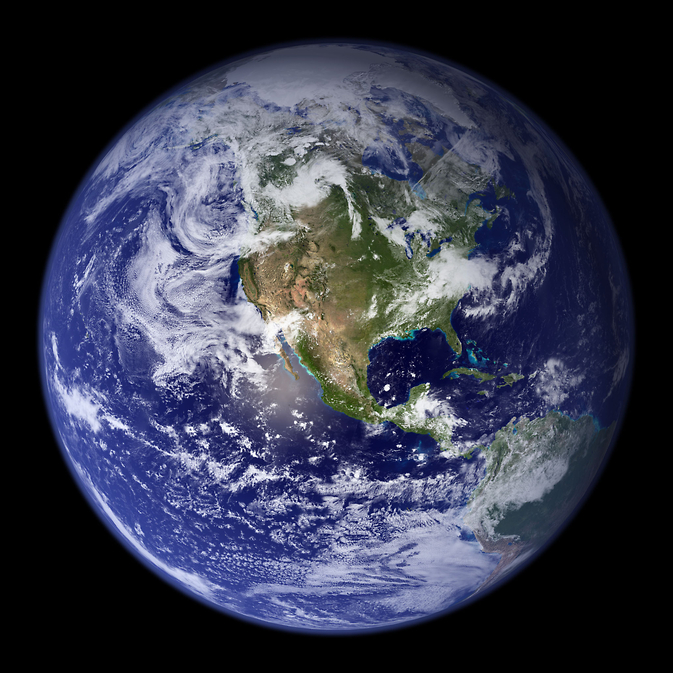
The components interact with each other by exchanging energy, water, momentum, and carbon thus creating a deliciously complex coupled system. Imagine water evaporating from the tropical ocean heated by the sun (Fig. 1). The air containing that water rises and cools. The water condenses into a cloud. The cloud is carried by winds over land where it rains. The rain sustains a forest. Trees are dark, having a low albedo. This influences the amount of sunlight absorbed by the Earth. Dark surfaces absorb more sunlight and get warmer compared to bright surfaces such as desert sand or snow. Air warmed by the surface rises and affects the wind.
d) Processes
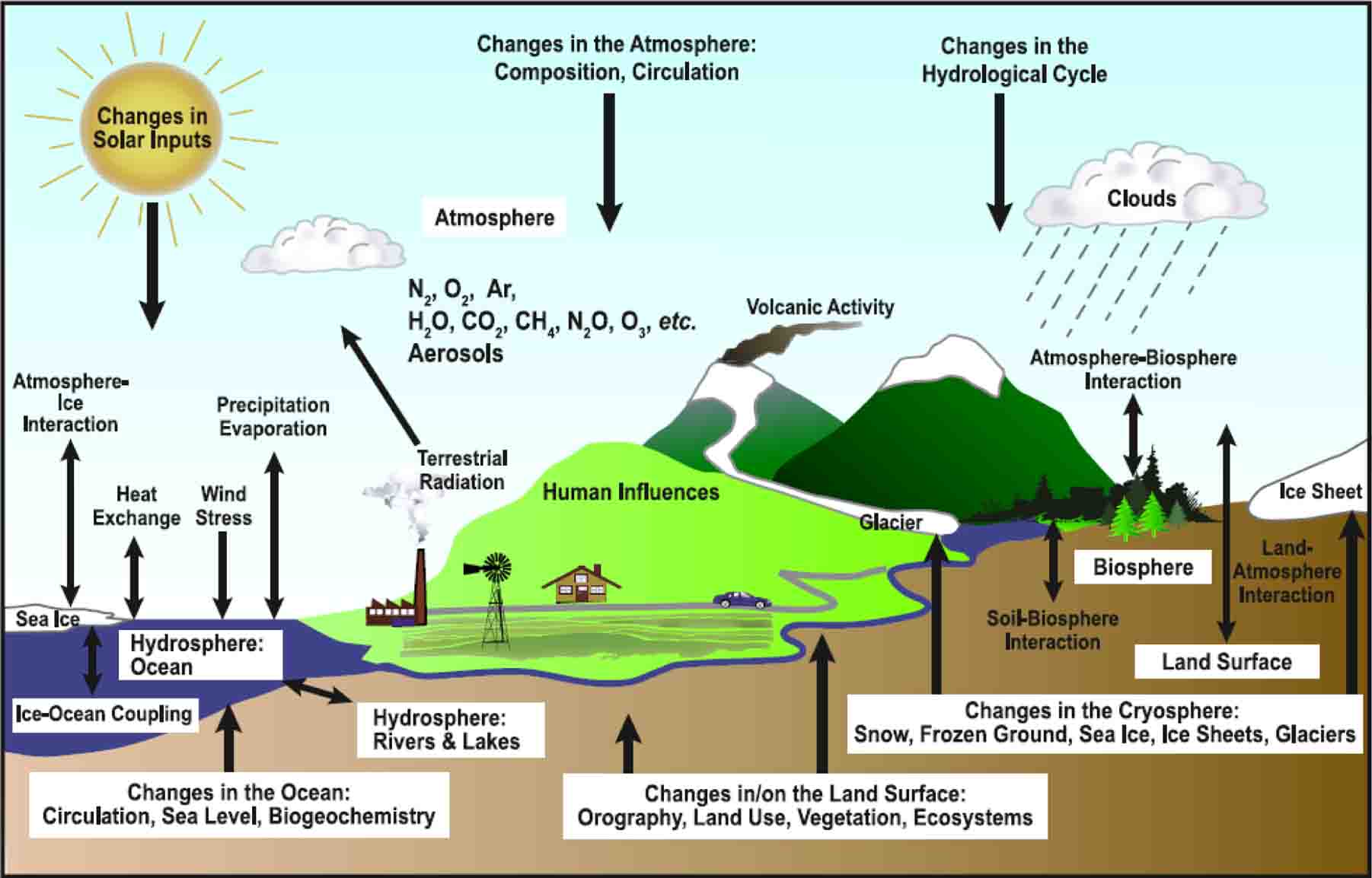
Fig. 2 illustrates some of the important processes that contribute to the complex interactions within the climate system. Earth’s energy source is the sun. Both solar and terrestrial radiation are affected by gases, aerosols, and clouds in the atmosphere. Thus, the atmospheric composition affects the heating and cooling of the earth. Heating and cooling affect the temperature and circulation of the atmosphere and oceans. Circulations of the air and sea affect temperatures and precipitation over both ocean and land, which impact the biosphere and cryosphere. Atmosphere and oceans exchange heat, water (evaporation and precipitation), and momentum. Wind blowing over the ocean pushes the surface water ahead. Air temperatures and snow fall affect the growth and melting of glaciers and ice sheets. Water from melting ice flows through rivers into the ocean affecting its salinity, its density and movement. Variations in solar irradiance can cause global climate to change. Volcanoes can eject large amounts of aerosol into the atmosphere with climatic implications. Humans are influencing the climate system through emissions of greenhouse gases, aerosols, and land use changes.
The complexity makes studying the climate system challenging. Scientists from many disciplines contribute such as physicists, chemists, biologists, geologists, oceanographers, atmospheric scientists, paleoclimatologists, mathematicians, statisticians, and computer scientists. To me, the challenges and interdisciplinary nature of climate science are fascinating and fun. I learn something new about it every day.
Recorded Lectures
References
Le Treut, H., R. Somerville, U. Cubasch, Y. Ding, C. Mauritzen, A. Mokssit, T. Peterson and M. Prather, 2007: Historical Overview of Climate Change. In: Climate Change 2007: The Physical Science Basis. Contribution of Working Group I to the Fourth Assessment Report of the Intergovernmental Panel on Climate Change [Solomon, S., D. Qin, M. Manning, Z. Chen, M. Marquis, K.B. Averyt, M. Tignor and H.L. Miller (eds.)]. Cambridge University Press, Cambridge, United Kingdom and New York, NY, USA.
Questions
- What are the two main differences between weather and climate?
- How big is Earth? How thick is the atmosphere, how deep the ocean?
- What are the components of Earth’s climate system?
- List processes that cause interactions between the components: atmosphere-ocean, atmosphere-biosphere, atmosphere-cryosphere, ocean-biosphere, ocean-cryosphere.
- Name three processes (forcings) that can cause global climate to change.
Explore
Go to one of the following websites and explore temporal variations of surface temperature observations in a location of your interest. Plot today’s data, yesterday’s, last week’s, last month’s, last year’s, the last decade’s, as far back as you can and make some notes on what you observe. Note regular, predictable cycles such as the diurnal and annual cycle in contrast with irregular, unpredictable variations such as day-to-day and year-to-year fluctuations. What causes the regular cycles? Try to order the variations with respect to their amplitude (strength). Discuss with fellow students and instructor.
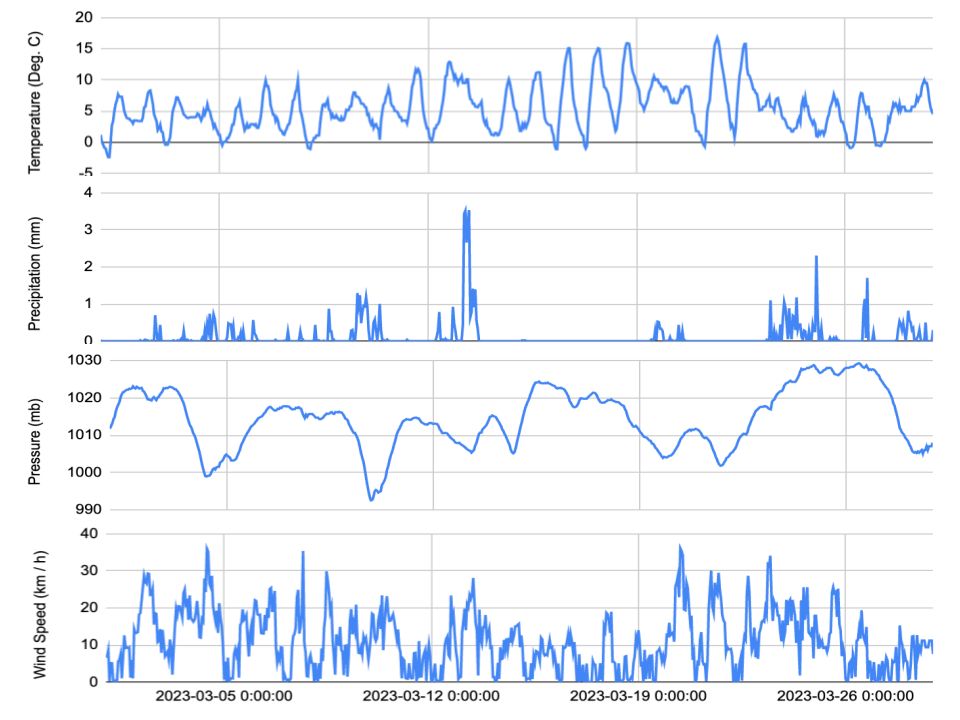
Hourly and daily data are available at visualcrossing.com. Enter a location of your interest and select “history” to get recent data. At the next step you can select different time periods. Unfortunately, hourly data are not shown for periods longer than 3 days, but you can sign up and download the data and plot them yourself. This is what I did below in Figure 3. I plotted them using Google Sheets. Are you able to identify diurnal (daily) cycles in temperature? Although some nights can be warmer than some days and sometimes days and nights have similar temperatures, on average days are warmer than nights. Thus the average diurnal cycle is part of climate. It is forced by the diurnal cycle of solar irradiance. Does pressure have a diurnal cycle? Answer: no. What is the typical timescale of pressure variations? Often it is about a week or so. This timescale is associated with the transition of weather systems (high and low pressure systems) passing by.
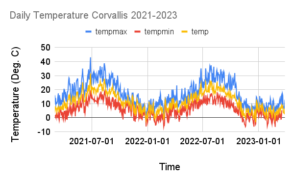
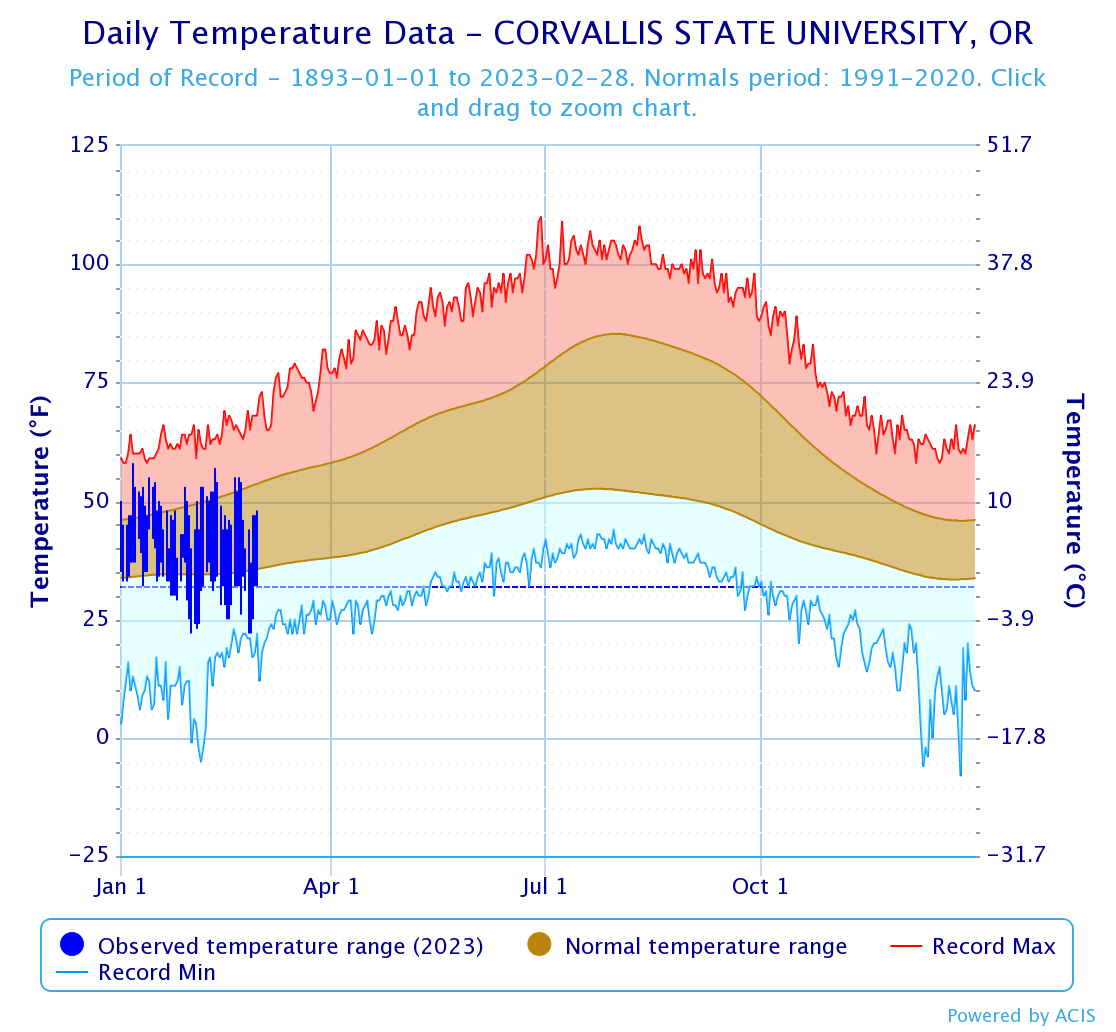
Daily temperature data are usually reported as a daily maximum, a daily minimum and an average. An example for Corvallis is shown in Fig. 4. It shows a clear seasonal cycle with temperatures in winter colder than in summer (duh).
Averaging many years of these weather data yields a climatology. For Corvallis it shows average temperatures around 40°F (4°C) in winter and 65°F (18°C) in summer (Fig. 5). It also shows a larger diurnal cycle in summer than in winter. What could be the reason for that? Answer: less cloud cover in summer. Clouds lead to cooler days and warmer nights, thus decreasing the diurnal cycle. Curves are smooth in the climatology. In contrast to Fig. 4 the weather variations have been averaged out.
Now try a forecast of temperature for next August and next January. What is your guess? Answer: a good guess would be the climatology, i.e. 65°F for August and 40°F for January. Thus the average seasonal cycle is climate and it is predictable because it is forced by the seasonal cycle of solar radiation. However, deviations from the climatology for a certain day next year are unpredictable weather.
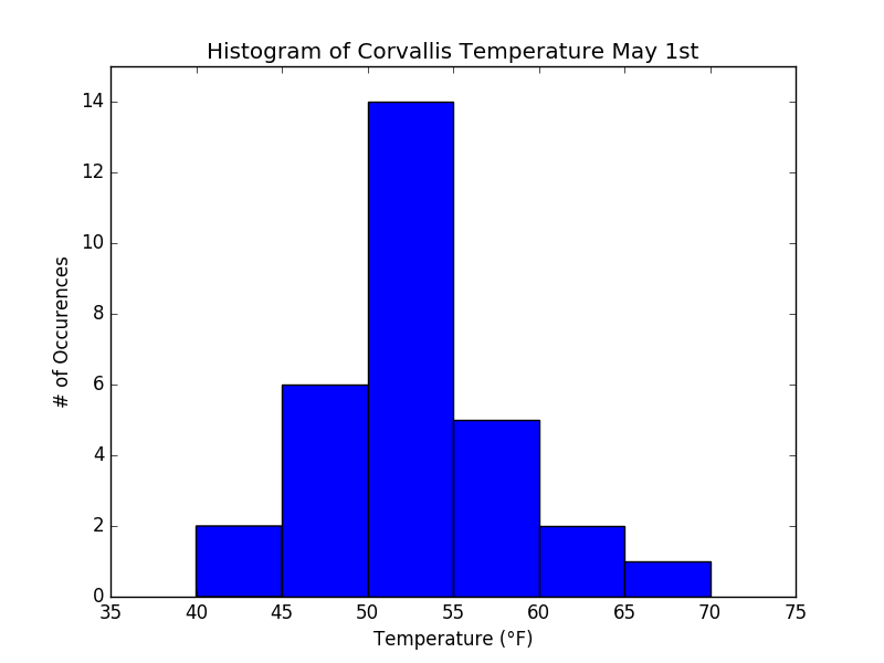
Statistical properties of climate can be summarized in a frequency histogram. Let’s explore those with an example. I have downloaded daily average temperature data from May 1st from 1985 to 2016. The following list (or vector mathematically speaking) of 30 years (N=30) of temperature data T = (T1, T2, … , TN) = (52, 52, 44, 52, 52, 54, 48, 52, 50, 56, 59, 46, 64, 58, 55, 48, 54, 54, 63, 54, 51, 54, 42, 52, 52, 48, 48, 48, 66, 56). Here N = 1 corresponds to 1985, N = 2 to 1986 and so on. In order to construct the frequency histogram we first need to choose bin sizes. I propose to choose 6 bins: 40-44, 45-49, 50-54, 55-59, 60-64, and 65-70. Now simply count how many years fall into each bin. I get 2, 6, 14, 6, 2, 1. Using python I produced the following graph (Fig. 6).
Climate change can be expressed as a change in the mean, which would correspond simply to a shift of the whole histogram to warmer or colder temperatures. However, it can also change the shape of the histogram. For example by making the distribution wider or narrower. This would increase or decrease the occurrences of extreme events. And, of course, it can both change the mean and the width. Most of the time, including in this text, discussions of climate change consider only changes in the mean. But we should keep in mind that changes to the tails of the distribution may be equally important because it is those tails that can have large impacts (heat waves, cold spells, droughts, floods, etc).
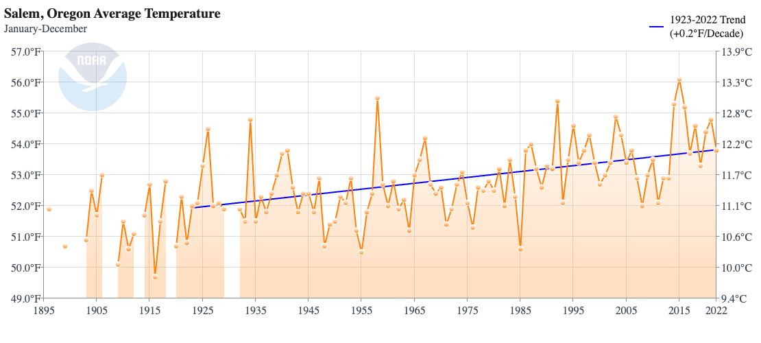
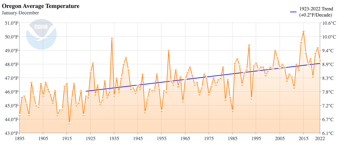
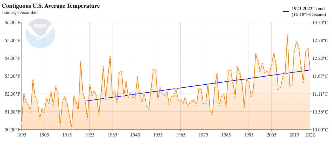
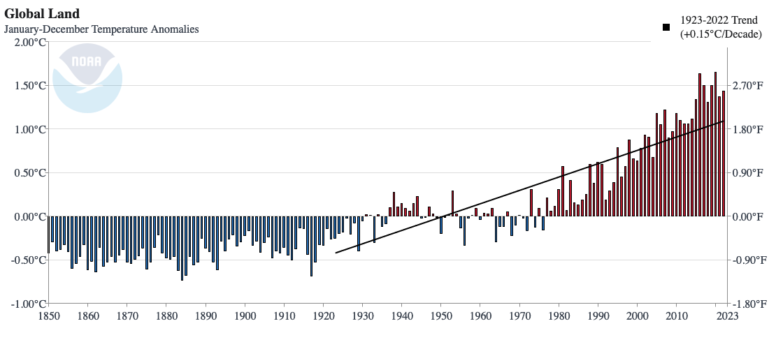
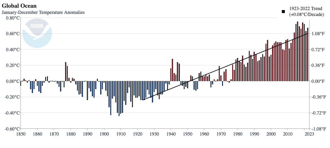
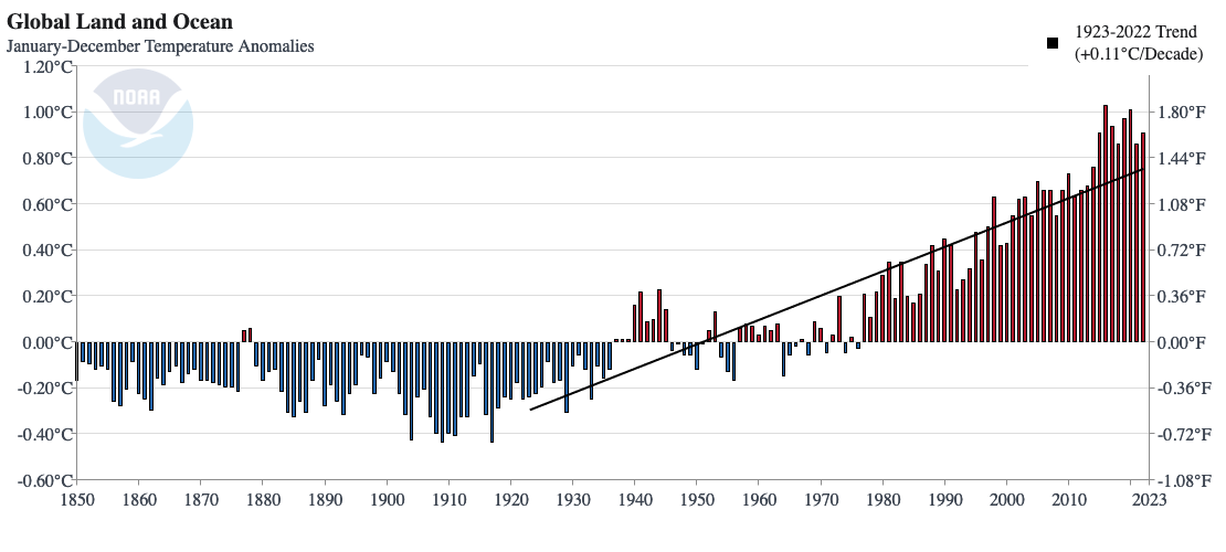
Now let’s explore effects of spatial scales on climate variations. Go to NOAA’s Climate-At-A-Glance website and start with the city tab selection. We want to compare the annual average temperature change in a city of your choice (e.g. Salem in Oregon), averaged over the larger region of a state, for the U.S. as a whole, and the globe. Use the “City Mapping” tab to select a city. For “Timescale” select “Annual”. Check the “Display Trend” box. This will include a trend line on the graph. Compare the trends and year-to-year variations. Are the trends larger for the global ocean or for the global land?
Compare the year-to-year variations and trends in regionally and globally averaged temperatures (Figs. 7-12) to the local diurnal cycle, day-to-day weather fluctuations (Fig. 3), and to the seasonal cycle (Figs. 4-5). Even though the global temperature trends (~0.1°C/decade) are much smaller than diurnal, day-to-day or seasonal fluctuations, which can be 10°C or more, we will see in the remainder of this course that global temperature changes of a few degrees C will have important impacts on natural systems and human societies.
- The weight of the ice depresses the lithosphere, which provides a feedback to the ice by lowering its surface elevation. Traditionally it has been thought that this feedback acts on long (millennial and longer) timescales, but recent research indicates that in certain regions such as West Antarctica, where the lithosphere is thin and the mantle viscosity is low the lithosphere can respond on much shorter (decadal to centennial) timescales. ↵
Rare weather or climate events such as hurricanes, typhoons, floods, droughts, and tornadoes that can often be damaging.
Reflectivity. Snow, ice, clouds and other bright surfaces have a high albedo, which leads to most sunlight being reflected to space. Ocean and vegetation on land have low albedos. They absorb lots of the suns radiation, which leads to warming.
Small particles in the air. Aerosols reflect sunlight back to space and therefore lead to cooling of the surface (negative forcing). Aerosols originate from natural (dust, ash from volcanic eruptions, wave breaking) and anthropogenic (smoke) sources.
Greenhouse gases are molecules that are able to absorb and emit electromagnetic radiation in the infrared part of the spectrum (longwave). Water vapor (H2O), carbon dioxide (CO2), methane (CH4), and nitrous oxide (N2O) are Earth’s most important greenhouse gases.
Humans' effects on the climate system through modifications of the land surface e.g. through deforestation and agriculture.
Radiative forcing (ΔF) is a change in energy fluxes F (in W/m2) at the top-of-the-atmosphere that causes climate change. It is defined as positive (negative) if it leads to warming (cooling). The radiative forcing for a doubling of CO2 is ΔF2xCO2 = 3.7 W/m2. Other examples are increased solar radiation (positive), increased aerosols (negative) or increased surface albedo (negative), e.g. due to land use changes.
