Climate models are tools used in climate research. They are attempts to synthesize our theoretical and empirical knowledge of the climate system in a computer code. This chapter describes how climate models are constructed, and how they are evaluated, and it discusses some applications.

a) Construction

Climate models solve budget equations numerically on a computer. The equations are based on the conservation of energy, momentum, and mass (air, water, carbon, and other relevant elements, substances, and tracers). Typically they are solved in separate boxes that represent specific regions of Earth’s climate system components (Fig. 1). Across their boundaries, the boxes exchange energy, momentum, and mass. Exchange with the flow of water or air from one box to another is called advection. Prognostic variables such as temperature, specific humidity in the atmosphere, or salinity in the ocean, and three velocity components (zonal, meridional, and vertical) are calculated in each box. The momentum equations, which are used to calculate the velocities, are based on Newton’s laws of motion and they include effects of the rotating Earth such as the Coriolis force. The temperature equations are based on the laws of thermodynamics. Thus, climate models represent the fundamental laws of physics as applied to Earth’s climate system.

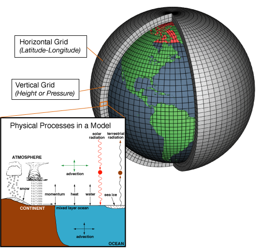
The evolution of the prognostic variables in the interior boxes are solved one time step at a time (see chapter 4, equation B1.4). After the prognostic variables have been updated the fluxes between boxes (I and O) are calculated, which are used for the next time step. Then the prognostic variables are updated again using the fluxes, and so on. This procedure is called forward modeling because all model variables at the next time step are calculated only from the model variables at the previous time step and the boundary conditions without the use of observations. Boundary conditions such as the incident solar radiation at the top-of-the-atmosphere or concentrations of greenhouse gases are usually required as input to the calculations. These are also called radiative forcings. Other boundary conditions need to be applied at the lower boundary: the topography (mountains) and bathymetry (sea floor). To start a forward model simulation initial conditions need also to be provided. Those can be taken from observations or idealized distributions.

Climate models range from the simplest zero-dimensional (0D) Energy Balance Model (EBM) discussed in chapter 4 to the most complex three-dimensional General Circulation Models (GCMs). The range of models ordered with respect to complexity is called the hierarchy of climate models. The 0D-EBM can be expanded by solving the energy budget equation separately at different latitudinal bands. This is called the one-dimensional EBM (1D-EBM). The 1D-EBM is still vertically averaged but it includes energy exchange between latitudinal bands as discussed in chapter 6. Meridional energy transport in 1D-EBMs is typically treated as a diffusive process proportional to the temperature gradient, such that heat flows from warm to cold regions. 1D-EBMs typically treat the ocean and atmosphere as one box, so that one cannot distinguish between heat transport in the ocean and atmosphere.

One-dimensional models are also used for vertical energy transfer in the atmosphere. These are called radiative-convective models and they work similar to the models used to produce Fig. (6) in chapter 4. Radiative-convective models themselves range in complexity from line-by-line models, which calculate radiative transfer in the atmosphere at individual wavelengths, to models that average over a range of frequencies (band models). Line-by-line models are computationally expensive and cannot be used in three-dimensional GCMs, which use band models. Band models are calibrated and tested by comparison to line-by-line models. As discussed in chapter 4, radiative fluxes alone would cause a much warmer surface and much colder upper troposphere than observed. Therefore, radiative-convective models include convection, mostly by limiting the lapse rate to the observed or moist adiabatic rate.

Intermediate complexity models consist of 2D-EBMs, which are still vertically averaged but include zonal transport of energy and moisture (in this case they are called Energy-Moisture-Balance Models or EMBMs), zonally-averaged ocean models coupled to a 1D-EBM, and zonally averaged dynamical atmospheric models (resolving the Hadley circulation). Intermediate complexity models also often include biogeochemistry and land ice components. They are computationally relatively inexpensive and can be run for many thousands or even millions of years.

The first climate models developed in the 1960s were 1D-EBMs and simple GCMs of the atmosphere and ocean at very coarse resolution. Initially ocean and atmospheric models were developed separately and only later they were coupled. Coupling involves the exchange of heat and water fluxes and momentum at the surface. Current state-of-the-science coupled, three-dimensional GCMs also include sea ice and land surface processes such as snow cover, soil moisture and runoff of water through river drainage basins into the ocean. Many models also include dynamic vegetation with separate plant functional types such as trees and grasses. However, most current coupled GCMs that are used for future projections do not include interactive ice sheet components. This is because ice sheets have long equilibration (response) times of tens of thousands of years and therefore they need to be run for a much longer time than the other climate system components, which is currently not possible for most climate models.

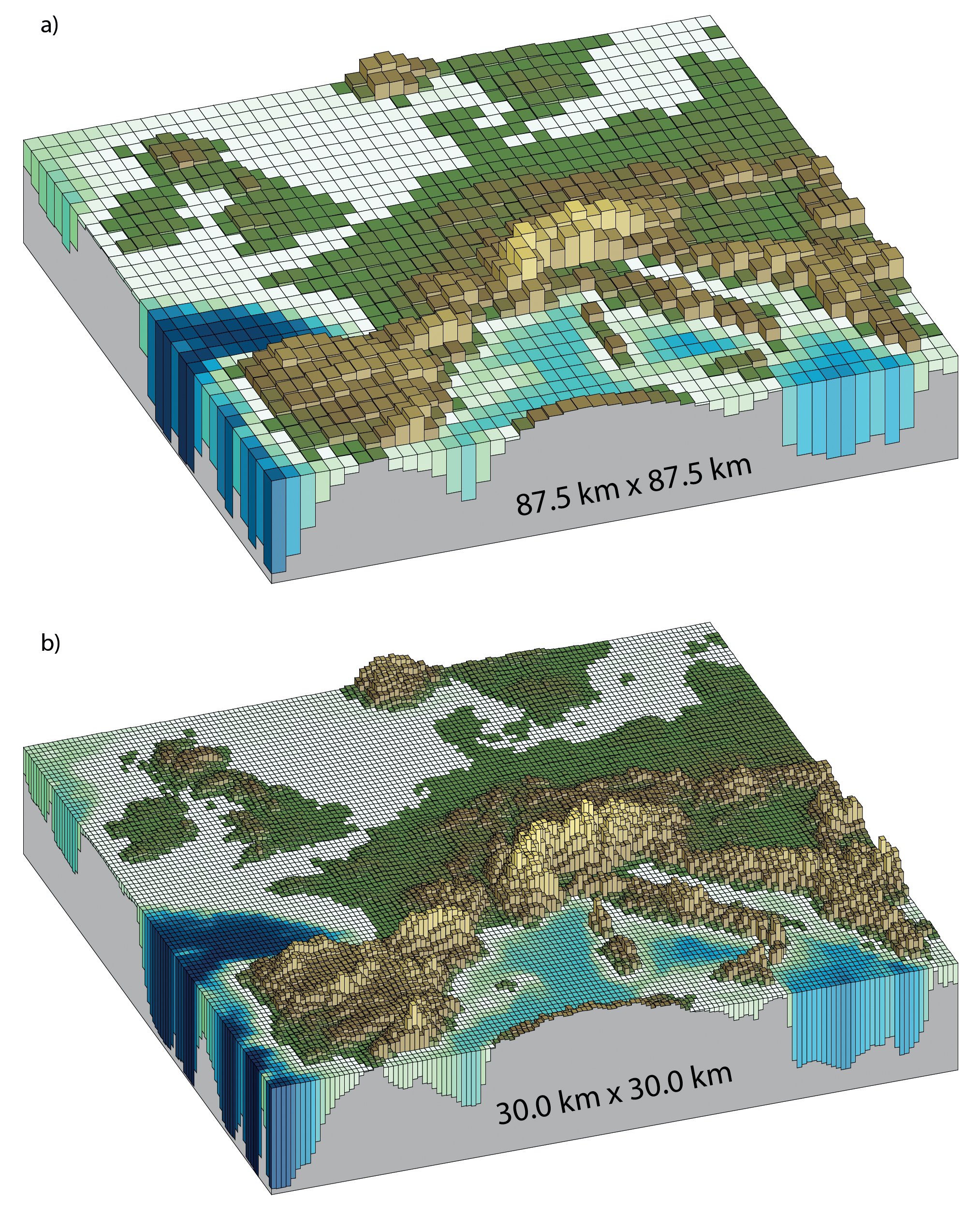
The deep ocean has an equilibration time of about a thousand years. For future projections people are mostly interested in the next hundred or perhaps a few hundreds of years. For the most reliable and detailed projections on these timescales global climate modeling groups try to configure their models at the finest possible resolution. Currently the typical resolution is a few degrees (~200 km) in the horizontal directions and 20 to 30 vertical levels each in the atmosphere and ocean components. Finer resolution global models are being developed at various climate modeling centers around the world, but currently most climate projections of centennial and longer time scales are based on coarser resolution models (Fig. 2).

Ice sheet models have finer spatial resolution (10s of kilometers) in order to resolve the narrow and steep ice sheet margin, but they have much larger time steps (1 year) than atmospheric (seconds) and ocean (minutes to hours) models because of the slow ice velocities (10-100 m/yr) compared to velocities of ocean currents (1-10 cm/s) or winds (1-10 m/s). The time step in a model depends on the velocity of the fluid and the grid-box size. The higher the velocity and the smaller the grid-box size the smaller the time step has to be to guarantee numerical stability. Finer resolution models therefore have to use smaller time steps, which is an additional burden on the computational resources. Another obstacle to move to higher resolution is the amount of data that accumulate. The highest resolution ocean model simulations currently require petabytes (10¹⁵ bytes = 1000 terrabytes) of storage for all the model output. Processing these huge amounts of data is a challenge.

One way to avoid increasing computational resources at higher resolution is to construct regional climate models for a specific region of interest, e.g. North America. However, the disadvantage of regional climate models is that boundary conditions at the margins of the model domain have to be prescribed. The resulting solution in the interior depends strongly on those boundary conditions, which often are taken from global climate models. Therefore, any bias from the global climate model at the boundary would be propagated by the regional model into the interior of the model domain. However, in the interior the regional climate model can account for details e.g. of the topography, that a global model cannot. Thus, although not a silver bullet, regional climate models are useful for simulating climate in more spatial detail than possible with global models.

Typically the resolution and grids of the atmospheric and ocean components are different. Therefore, surface fluxes and variables needed to calculate the fluxes need to be mapped from one grid to the other. This is often accomplished by a coupler, which is software that does interpolation, extrapolation, and conservative mapping. All calculations need to be numerically sound such that energy, water, and other properties are conserved. However, numerical schemes, e.g. for the transport from one box to the next, are associated with errors and artifacts.

Models that include biogeochemistry, such as the carbon cycle, and/or ice sheets are called Earth System Models. Earth System Models calculate atmospheric CO₂ concentrations interactively based on changes in land and ocean carbon stocks. They can be forced directly with emissions of anthropogenic carbon, whereas models without carbon cycles need to be forced with prescribed atmospheric CO₂ concentrations.

Due to the limited resolution of the models, processes at spatial scales below the grid box size cannot be directly simulated. For example, individual clouds or convective updrafts in the atmosphere are often only a few tens or hundred meters in size and therefore cannot be resolved in global atmospheric models. Similarly, turbulence and eddies in the ocean, which are important for the transport of heat and other properties, cannot be resolved by global ocean models. These processes must be parameterized. A parameterization is a mathematical description of the process that depends on the resolved variables, e.g. the mean temperature in the grid box, and one or more parameters. A simple example of a parameterization is the meridional heat flux F_m = -K∂T/∂y in a 1D-EBM, which can be parameterized as a diffusive process, where K>0 is the diffusivity, ∂T/∂y is the meridional temperature gradient and y represents latitude. This parameterization transports heat down-gradient (note the minus sign), which means from warmer to colder regions. In this case the parameter K can be determined from observations of meridional heat flux (Chapter 6, Fig. 4) and ∂T/∂y (Chapter 6, Fig. 1). Parameterizations can be derived from empirical relationships based on detailed measurements or high-resolution model results. The parameter values are usually not precisely known but they influence the results of the climate model. Therefore, parameterizations are a source of error and uncertainty in climate models. Parameters in the cloud parameterization of a model, for example, will impact its cloud feedback and therefore its climate sensitivity.

b) Evaluation

Climate models are evaluated by comparing their output to observations. Figs. 3 & 4 show the multi model mean (the average of all models) from the IPCC’s 6th Assessment Report (AR6). The modeled surface temperature distribution is similar to the observations (Chapter 6, Fig. 1) with warm (20-30°C) temperatures in the tropics and cold (<0°C) temperatures near the poles and at high altitudes (Himalayas). The models also reproduce some of the observed zonal gradients such as the cooler temperatures in the eastern equatorial Pacific compared to the western Pacific warm pool and the warmer temperatures in the northeast Atlantic compared to the northwest Atlantic, which are caused by the upper ocean circulation. However, the models are not perfect, as indicated by biases such as too warm temperatures in the southeast Atlantic and Pacific. Those warm biases are most likely caused by the coarse resolution ocean model components that do not resolve well the narrow upwelling in these regions. A similar bias is seen in the California current in the northeast Pacific. Another region where the models are collectively too warm is the Atlantic and Indian ocean sections of the Southern Ocean, perhaps related to issues in reproducing clouds there. Despite these biases the multi model mean agrees with the observed temperatures to within plus/minus one degree Celsius in most regions. Even the larger regional biases such as those mentioned above are relatively small compared to the ~60°C range of temperature variations on Earth. This, and the fact that the bias is significant in only relatively small areas in Fig. 3 (not hatched), indicates that the models reproduce observed surface temperatures relatively well.

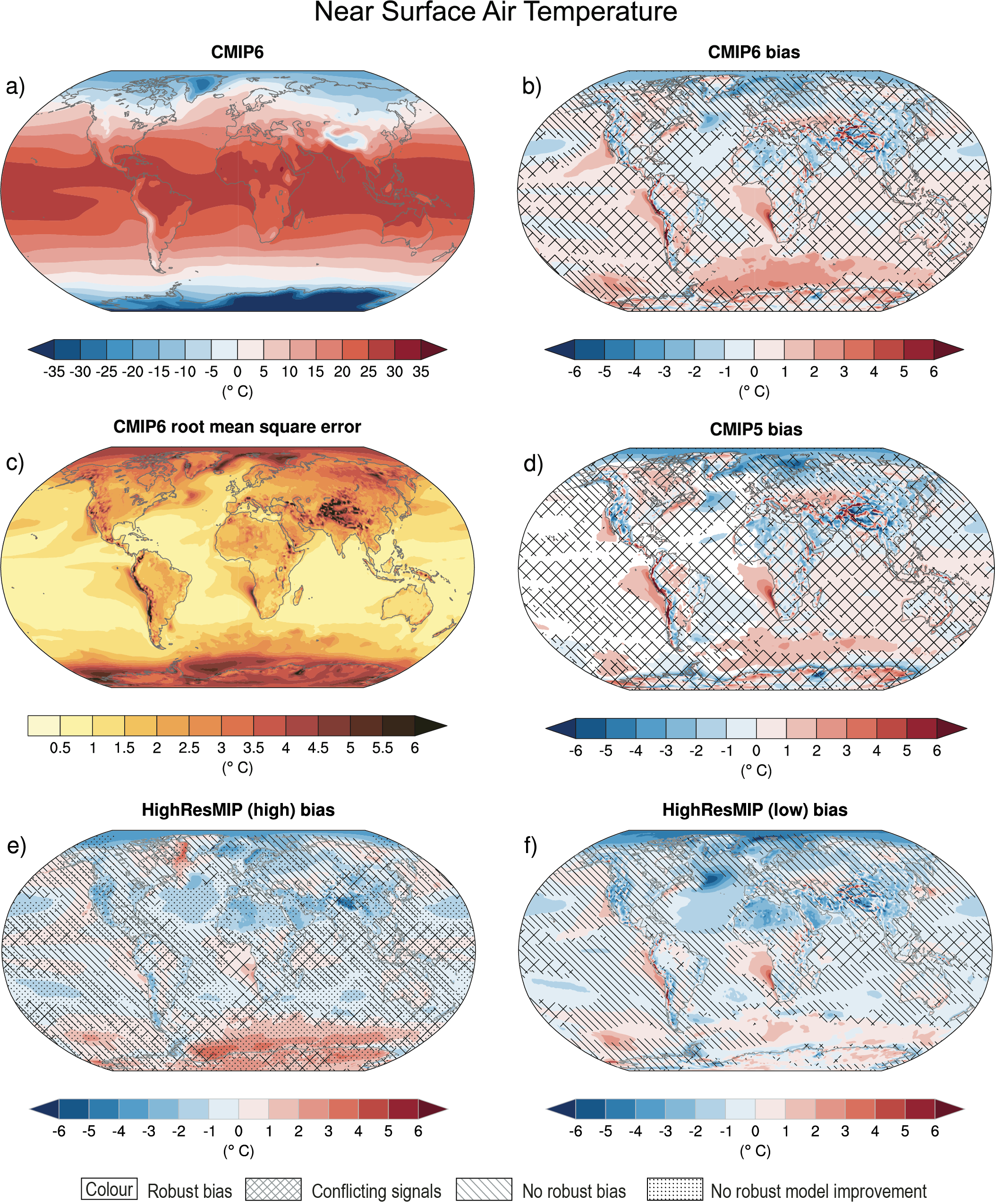
Fig. 4 shows the multi model mean precipitation. The models reproduce the general pattern of the observations (Chapter 6, Fig. 8) such as more precipitation in the tropics and at mid-latitudes compared with less precipitation in the subtropics and at the poles. They also reproduce some of the observed zonal differences such as dryer conditions over the eastern parts of the subtropical ocean basins compared with wetter conditions further west. However, the models also display systematic biases such as the double Intertropical Convergence Zone (ITCZ) over the East Pacific and too dry conditions over the Amazon. The relative errors in precipitation are generally larger than those for temperature. This, and the larger non-hatched area in Fig. 4 compared with Fig. 3, indicates that the models are better in simulating temperature than precipitation. This may not be surprising given that the simulation of precipitation depends strongly on parameterized processes such as convection and clouds.

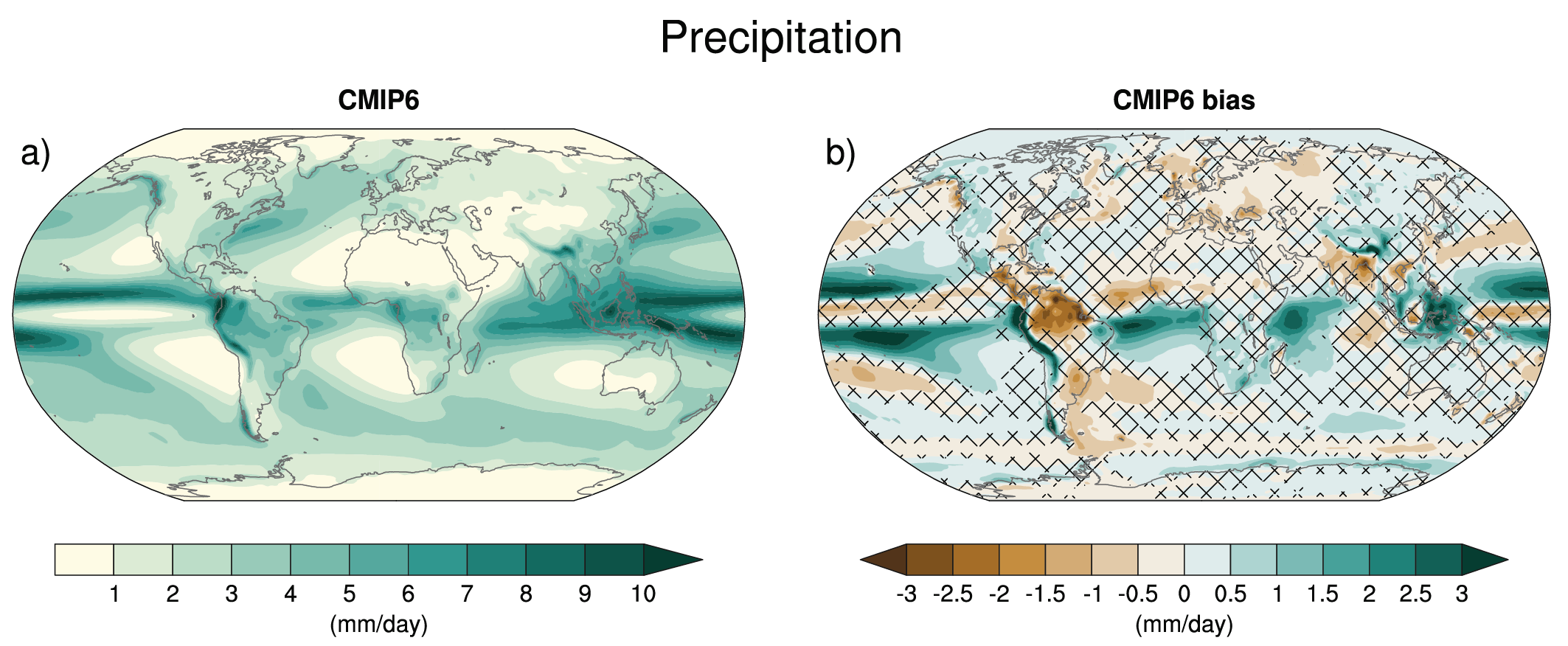
Fig. 5 compares correlation coefficients of different variables. It confirms our previous conclusion that the models are better in simulating temperature than precipitation, although it also indicates considerable uncertainty in the observations for precipitation. It also shows that the models have very good skill in simulating Emitted Terrestrial Radiation at the top-of-the-atmosphere^[1], whereas they are less good at simulating clouds and associated Reflected Solar Radiation^[2]. The most recent generation of climate models (CMIP6) has improved compared with previous generations (CMIP5 and CMIP3) particularly for precipitation, clouds and shortwave fluxes.

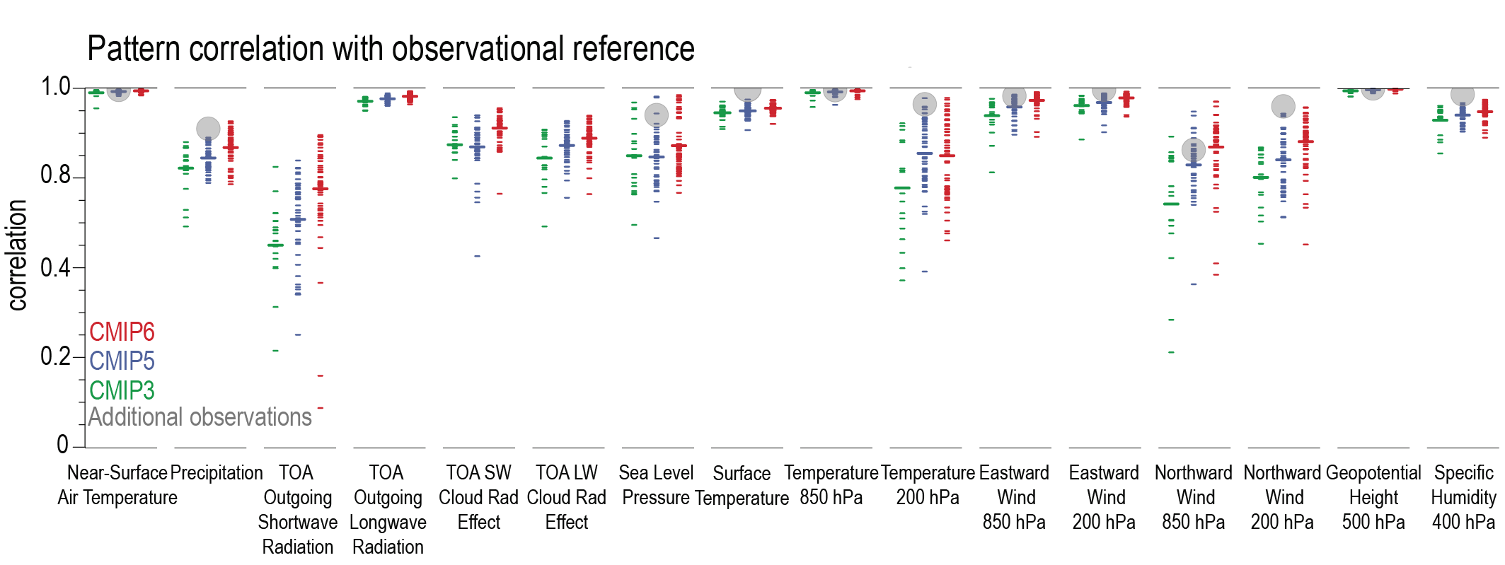
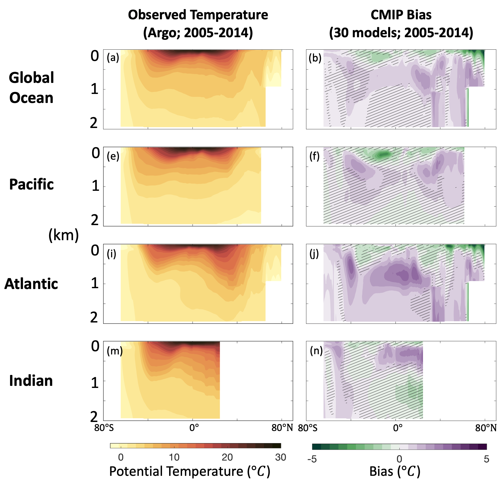
Fig. 6 shows that the models also reproduce the observed distribution of subsurface temperatures in the ocean. Remaining model biases are overestimated temperatures in the tropical Atlantic and Indian ocean thermocline by 1-2°C. Again these errors are relatively small given the large range (~20°C) of subsurface ocean temperature variations. Model errors in salinity are larger near the surface than in the deep ocean. In the southern hemisphere subtropics near surface waters are too fresh, perhaps related to the double ITCZ bias and associated too wet conditions in the atmosphere there (Fig. 5).

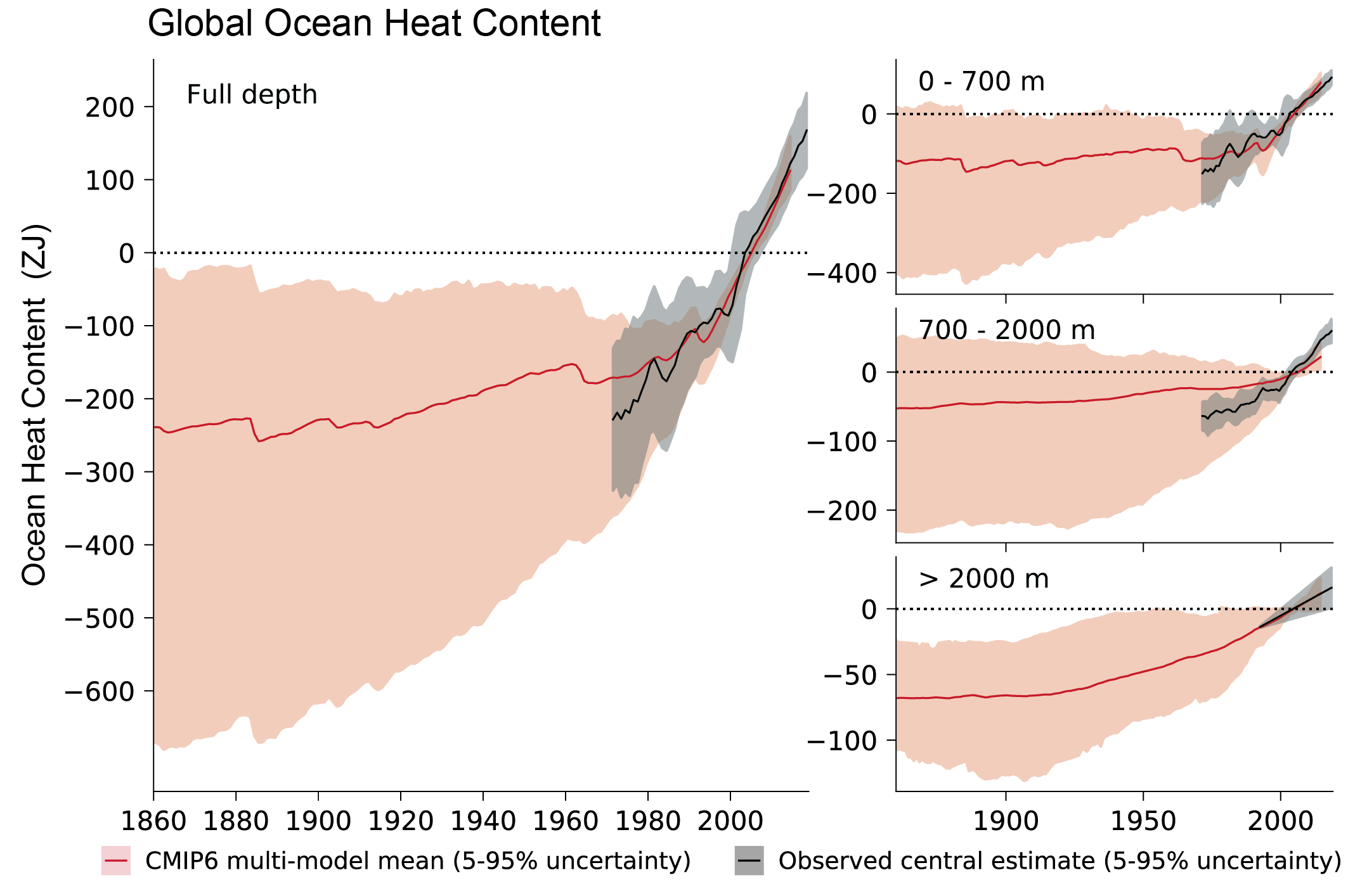
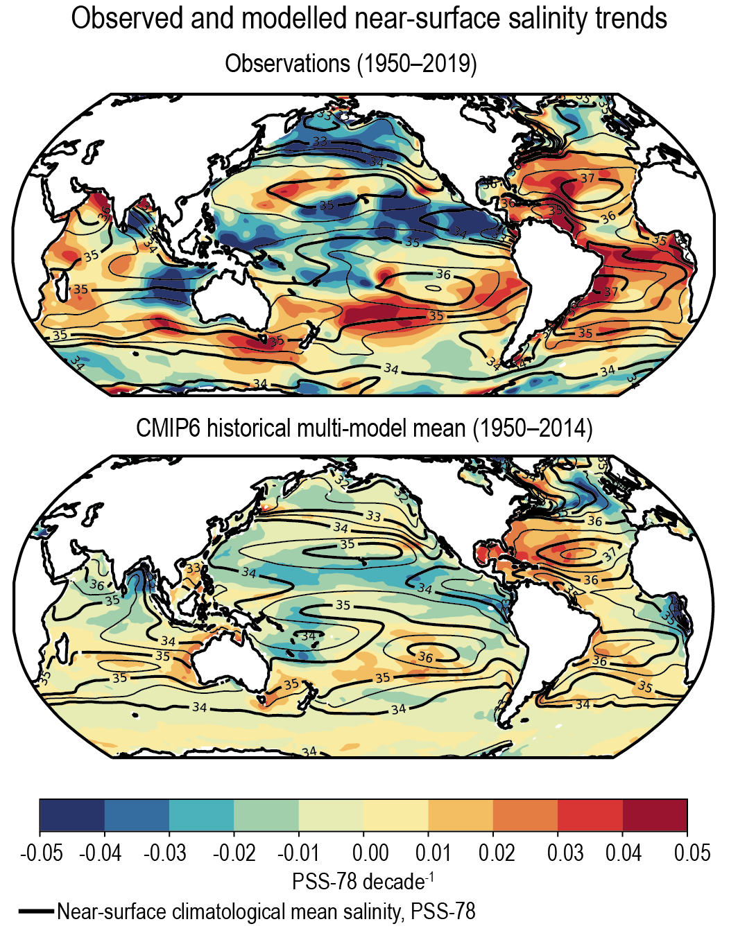
All climate models simulate an increasing ocean heat content over the last 40 years, consistent with observations (Fig. 7). Some models simulate more and others less heat uptake. The multi model mean, however, is in good agreement with the observations. This indicates that the models are skillful not only in simulating the mean state of ocean temperatures but also its recent temporal evolution. The observed patters of salinity changes are also well reproduced by the models as illustrated in this figure.

Historical and paleoclimate variations are also used to test and evaluate climate models as will be discussed next.

c) Applications

Some of the main applications of climate models are paleoclimate studies, detection and attribution studies, and future projections. Future projections will be discussed in the next chapter.

Paleoclimate model studies are not only useful for a better understanding of past climate changes and their impacts but they can also be used to evaluate the models. For example, model simulations of the Last Glacial Maximum (LGM) are broadly consistent with temperature reconstructions (see Chapter 3) that show global cooling of 4-5°C, polar amplification and larger changes over land than over the ocean. The models reproduce these basic features of the reconstructions, which indicates that they have skill simulating climates different from the present (Masson-Delmotte et al., 2013). On the other hand, there are also differences between model results and observations, e.g. in deep ocean circulation (Muglia et al., 2015), which indicates that model’s skills in those aspects are questionable.

Detection and attribution studies attempt to determine which observed climate changes are unusual (detection) and what are its causes (attribution). Climate models driven with only natural forcings show variations from one year to the next due to internal climate variability (e.g. El Niño) and short term cooling in response to large volcanic eruptions (Fig. 8). However, they do not show a long-term warming trend over the past century, in contrast to the observations. This suggests that the global warming observed since about the 1970’s is highly unusual and cannot be explained by internal climate variability (as represented in the models) nor by natural drivers. However, if anthropogenic forcings are included the models reproduce very well the observed long term trend. The multi model mean also reproduces well the observed short term coolings associated with large volcanic eruptions of the past 50 years.

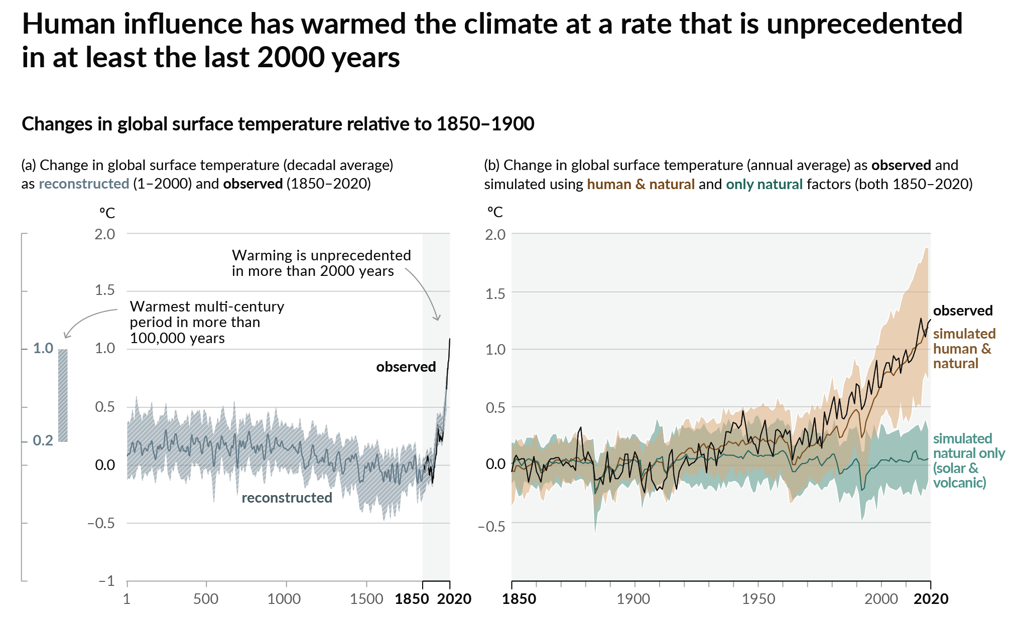
Models driven with both natural and anthropogenic forcings reproduce well not only the observed global mean temperature changes but also its spatial distribution (not shown) such as larger warming at high northern latitudes (polar amplification) and over land (land-sea contrast). These results represent evidence that human activities are the main reason for the observed warming during the past 50-60 years. The IPCC’s AR6 concludes that “it is unequivocal that human influence has warmed the atmosphere, ocean and land since pre-industrial times“(IPCC 2021).

Videos

Recorded Lecture: Climate Models

References

IPCC, 2021: Chapter 3. In: Climate Change 2021: The Physical Science Basis. Contribution of Working Group I to the Sixth Assessment Report of the Intergovernmental Panel on Climate Change [Eyring, V., N.P. Gillett, K.M. Achuta Rao, R. Barimalala, M. Barreiro Parrillo, N. Bellouin, C. Cassou, P.J. Durack, Y. Kosaka, S. McGregor, S. Min, O. Morgenstern, and Y. Sun, 2021: Human Influence on the Climate System. In Climate Change 2021: The Physical Science Basis. Contribution of Working Group I to the Sixth Assessment Report of the Intergovernmental Panel on Climate Change [Masson-Delmotte, V., P. Zhai, A. Pirani, S.L. Connors, C. Péan, S. Berger, N. Caud, Y. Chen, L. Goldfarb, M.I. Gomis, M. Huang, K. Leitzell, E. Lonnoy, J.B.R. Matthews, T.K. Maycock, T. Waterfield, O. Yelekçi, R. Yu, and B. Zhou (eds.)]. Cambridge University Press, Cambridge, United Kingdom and New York, NY, USA, pp. 423–552, doi: 10.1017/9781009157896.005 .]

Masson-Delmotte, V., M. Schulz, A. Abe-Ouchi, J. Beer, A. Ganopolski, J.F. González Rouco, E. Jansen, K. Lambeck, J. Luterbacher, T. Naish, T. Osborn, B. Otto-Bliesner, T. Quinn, R. Ramesh, M. Rojas, X. Shao and A. Timmermann, 2013: Information from Paleoclimate Archives. In: Climate Change 2013: The Physical Science Basis. Contribution of Working Group I to the Fifth Assessment Report of the Intergovernmental Panel on Climate Change [Stocker, T.F., D. Qin, G.-K. Plattner, M. Tignor, S.K. Allen, J. Boschung, A. Nauels, Y. Xia, V. Bex and P.M. Midgley (eds.)]. Cambridge University Press, Cambridge, United Kingdom and New York, NY, USA.

Muglia, J., and Schmittner, A. (2015) Glacial Atlantic overturning increased by wind stress in climate models, Geophysical Research Letters, 42, doi:10.1002/2015GL064583.